
Colab notebook:  Google Colab

TL;DR
- Bayesian ML treats model parameters as random variables, not fixed points. This allows us to reason about model uncertainty.
- The core workflow is Prior Belief + Data (Likelihood) → Posterior Belief.
- Maximum A Posteriori (MAP) is a simple bridge from classical ML, adding a prior term to Maximum Likelihood (MLE).
- For complex models, the posterior is intractable. We approximate it with MCMC (sampling) or Variational Inference (optimization).
- Modern techniques like the Reparameterization Trick and MC Dropout make it possible to train Bayesian Neural Networks at scale, providing principled uncertainty estimates for deep learning.
Roadmap
This tutorial builds a complete picture of modern Bayesian ML, from first principles to deep learning applications.
- Bayes’ Theorem & Priors: The fundamental rule for updating beliefs with evidence.
- Maximum Likelihood vs. Maximum A Posteriori: Contrasting point estimation methods to see how priors act as regularizers.
- Bayesian Linear Regression: Our first "fully Bayesian" model, moving from point estimates to parameter distributions.
- Monte Carlo Methods (MCMC): A class of algorithms for sampling from complex posterior distributions when closed-form solutions are impossible.
- ELBO (Evidence Lower Bound): The objective function at the heart of modern Variational Inference, trading sampling for optimization.
- Reparameterization Trick: The key mathematical device that allows us to train variational models with gradient descent.
- Bayesian Neural Networks: Extending Bayesian principles to deep learning by placing distributions over network weights.
- Dropout as Bayesian Approximation: A surprising and powerful connection that lets us get uncertainty from standard NNs.
1. Bayes’ Theorem & Priors
Concept: Bayesian inference is a framework for updating our beliefs in light of new evidence. It starts with a prior belief about a parameter, p(θ), which represents our knowledge before seeing any data. We then collect data D and define a likelihood, p(D|θ), a function that describes how probable the observed data is for a given value of the parameter θ. Bayes' theorem combines these two to give us the posterior distribution, p(θ|D), which represents our updated belief about θ after observing the data.
Equation: The theorem itself is elegant and foundational.
Here, p(D), the evidence (or marginal likelihood), acts as a normalization constant. It's the probability of observing the data averaged over all possible parameter values: p(D) = ∫ p(D|θ)p(θ)dθ. This integral is often the hardest part to compute, which motivates the approximation methods we'll see later.
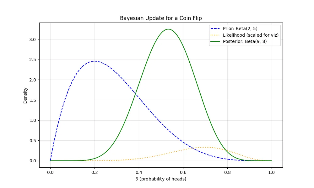
Figure 1: Visualizing a Bayesian Update
A simple model helps build intuition. Let's say we're modeling coin flips. Our parameter θ is the probability of heads. We can use a Beta distribution as our prior and a Bernoulli distribution as our likelihood. This is a "conjugate" pair, meaning the posterior is also a Beta distribution.
Experiment: Let's code this update. We start with a prior belief that the coin is slightly biased towards tails (α=2, β=5). We then observe 10 flips: 7 heads (H=7) and 3 tails (T=3)
2. Maximum Likelihood vs. Maximum A Posteriori
Concept: Most standard machine learning training is Maximum Likelihood Estimation (MLE). We find the parameters θ that make the observed data most probable. In the Bayesian world, a simple first step is Maximum A Posteriori (MAP) estimation. Instead of maximizing just the likelihood, we maximize the posterior probability. Because the evidence p(D) is constant with respect to θ, this is equivalent to maximizing the likelihood times the prior.
Equation: It's most common to work with log probabilities to turn products into sums.
The log p(θ) term is key. It's a regularizer. If our prior p(θ) is a Gaussian centered at zero, then log p(θ) becomes a term proportional to -||θ||², which is exactly L2 regularization!
Pitfall: The "regularization = log-prior" analogy is powerful but imperfect. It holds for simple cases, but the Bayesian approach is more general. The goal is to find a full posterior distribution, not just its mode (the peak). MAP, like MLE, gives only a single point estimate and discards all uncertainty.
Figure 2: The Geometry of MLE vs. MAP
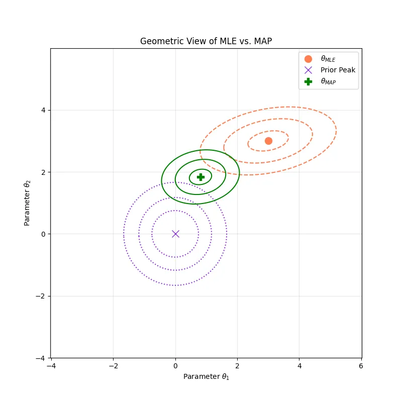
Experiment: Let's estimate the mean μ of a 1D Gaussian. The MLE estimate is simply the sample mean. We'll use a Gaussian prior on μ and see how it pulls the MAP estimate.
The strong prior N(0, 1) pulls the MAP estimate significantly away from the sample mean and towards zero. With a flatter prior (e.g., prior_sigma = 10), the MAP estimate would be much closer to the MLE.
3. Bayesian Linear Regression
Concept: Standard linear regression finds a single best-fit line by learning point estimates for weights w and bias b. Bayesian Linear Regression (BLR) takes this a step further. We place priors on w and b (usually Gaussians) and compute the full posterior distribution over them. This means that for any input x*, we don't get a single prediction y*; we get a full predictive distribution p(y*|x*, D). The mean of this distribution is our prediction, and its variance tells us our uncertainty.
Equation: For a Gaussian prior on weights w ~ N(0, α⁻¹I) and a Gaussian likelihood with precision β, the posterior for w is also a Gaussian, p(w|X, y) ~ N(m_N, S_N). The posterior predictive distribution is also a Gaussian, p(y*|x*, X, y) ~ N(m_Nᵀx*, σ²(x*)). The full equations for m_N, S_N, and σ²(x*) are in the appendix, but the key idea is they are solvable in closed form.
Experiment: We'll fit a BLR model to a noisy 1D sine wave. The plot will show not just the mean prediction, but also the uncertainty, which should be higher in regions with no data.
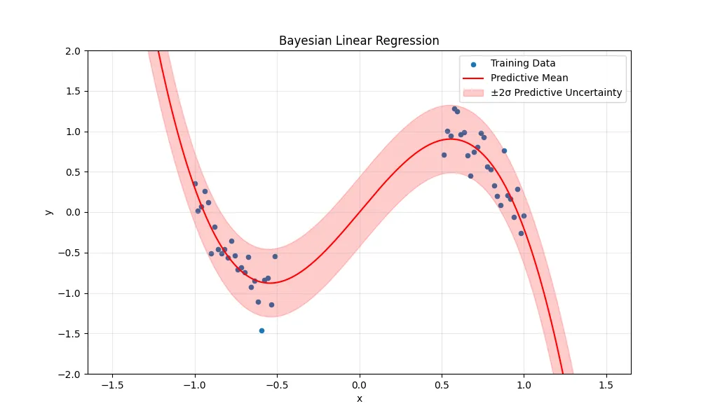
The shaded region shows the model's uncertainty. Notice how the uncertainty band widens dramatically in the gap between x = -0.5 and x = 0.5, where we have no data. This is a key advantage of the Bayesian approach: the model knows what it doesn't know.
4. Monte Carlo Methods (MCMC)
Concept: Bayesian Linear Regression is nice because its posterior is tractable. For most interesting models (like neural networks), the integral in the denominator of Bayes' rule is intractable. Monte Carlo (MC) methods are a class of algorithms that let us approximate an intractable posterior by drawing samples from it. The idea is that if we can draw enough representative samples {θ₁, θ₂, ..., θₙ} from p(θ|D), we can approximate any property of the posterior, like its mean or variance.
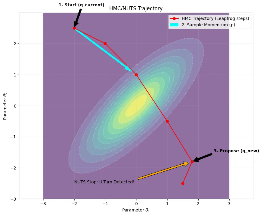
Markov Chain Monte Carlo (MCMC) algorithms like Metropolis-Hastings and Gibbs sampling construct a Markov chain whose stationary distribution is our target posterior. More advanced methods like Hamiltonian Monte Carlo (HMC) and its adaptive variant, the No-U-Turn Sampler (NUTS), use gradient information to propose samples more efficiently, making them the standard choice in modern probabilistic programming libraries like Stan or PyMC.
Diagram: HMC/NUTS Phase Space
Sanity Checks: Since MCMC is a stochastic process, we need to check if it worked. Two key diagnostics are:
- Effective Sample Size (ESS): Measures how many independent samples our correlated MCMC chain is worth. Low ESS means poor exploration.
- R-hat (R̂): Compares the variance between multiple parallel MCMC chains to the variance within each chain. An R̂ value close to 1.0 (e.g., < 1.01) suggests the chains have converged to the same distribution.
5. ELBO (Variational Inference)
Concept: MCMC can be very slow. Variational Inference (VI) reframes Bayesian inference as an optimization problem. Instead of sampling, we posit a family of simple, tractable distributions q(θ; λ) (e.g., Gaussians) indexed by parameters λ. We then try to find the parameters λ that make our "variational distribution" q as close as possible to the true posterior p(θ|D). The measure of "closeness" is the Kullback-Leibler (KL) divergence, KL(q || p). Minimizing this KL divergence is equivalent to maximizing a quantity called the Evidence Lower Bound (ELBO).
Equation Derivation: We start with the log evidence and apply some algebra.
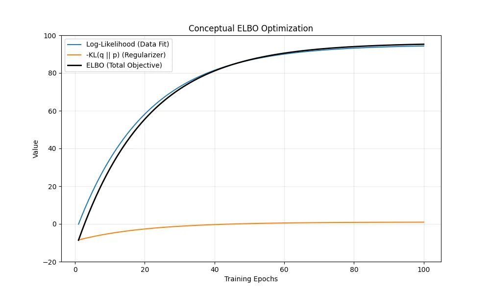
This final line is the ELBO. Maximizing it pushes q to explain the data (first term) while staying close to the prior (second term).
Table: The Two Faces of the ELBO
| Term | Role | Analogy |
|---|---|---|
| (Likelihood) | Data-fit / Reconstruction. Pushes the approximate posterior $q$ to put mass on parameters $\theta$ that explain the data well. | |
| (KL Regularizer) | Encourages the approximate posterior $q(\theta)$ to stay close to the prior $p(\theta)$. |
Experiment: We can't fit a full VI model here, but we can visualize the ELBO's components. Imagine a model with a reconstruction loss and a KL loss. During training, we are trying to maximize the sum of these two (or minimize the negative sum).
6. Reparameterization Trick
Concept: To optimize the ELBO with gradient descent, we need to differentiate it. The likelihood term is tricky because the expectation E_q depends on the parameters λ we want to optimize. How do you backpropagate through a sampling operation? The Reparameterization Trick is the solution. We rewrite the random variable θ ~ q(θ; λ) in a way that isolates the randomness.
Equation: For a Gaussian variational distribution q(θ; μ, σ) = N(θ | μ, σ²), instead of sampling θ directly, we sample a noise variable ε from a fixed distribution and then compute θ as a deterministic function.
Now, the stochastic part (ε) is outside the computational graph, and we can easily compute gradients of functions of θ with respect to μ and σ. This trick is fundamental to Variational Autoencoders (VAEs) and Bayesian Neural Networks.
Experiment: We will demonstrate that we can compute gradients for μ and σ after a sampling step. Note: Since torch.autograd is unavailable, this code is a conceptual demonstration of the data flow.
This confirms that gradients can be computed for the distribution's parameters (mu, log_sigma) even though z is a "random" sample.
7. Bayesian Neural Networks
Concept: A Bayesian Neural Network (BNN) is a neural network where we replace the point-estimate weights with distributions. Instead of a weight matrix W, we learn a posterior distribution p(W|D). For a simple BNN using Variational Inference, each weight w_ij is not a single number but is instead represented by parameters of its variational posterior, typically μ_ij and σ_ij for a Gaussian distribution.
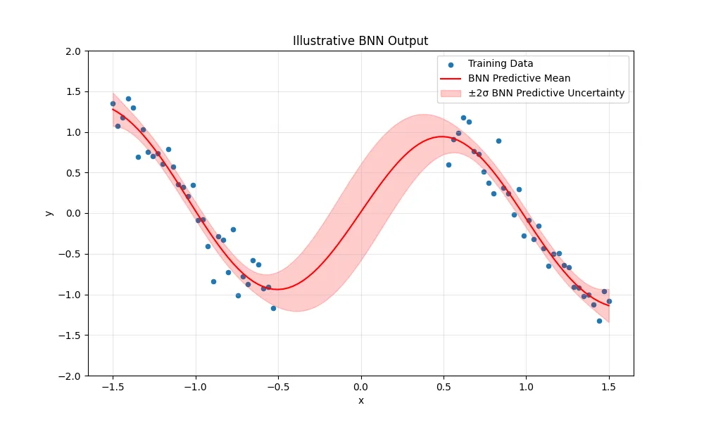
The training process involves optimizing the ELBO. The forward pass is different: for each training example, we sample a different set of weights from q(W) and pass the input through this sampled network. This naturally incorporates uncertainty and regularization.
Equation: The objective function is simply the ELBO, where θ is now the set of all network weights W. This is often called the "Bayes by Backprop" objective.
Here, λ represents all the learnable parameters of the weight distributions (all the μs and σs).
Experiment: Training a real BNN requires a framework like PyTorch. However, we can simulate its output. We'll take the same noisy sine wave data and plot what a trained BNN's predictions might look like. The key feature is that uncertainty increases where there is no data.
8. Dropout as Bayesian Approximation
Concept: This is one of the most remarkable and practical ideas in recent Bayesian ML. Gal and Ghahramani (2016) showed that a standard neural network with dropout, when dropout is also used at test time, can be interpreted as an approximation to a Bayesian neural network. The technique is called MC Dropout.
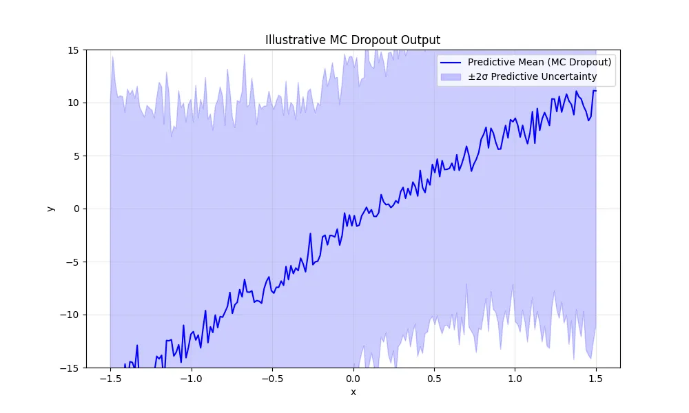
The procedure is simple: for a given test input x*, instead of just doing one forward pass with the final trained weights, you do T separate forward passes. In each pass, you use the same trained weights but a different random dropout mask. This gives you T different outputs {y*₁, y*₂, ..., y*ᵀ}. The sample mean of these outputs is your prediction, and their sample variance is your uncertainty estimate.
Experiment: We can implement this on a simple NumPy-based MLP. We'll define a standard MLP with ReLU activations and dropout layers. We'll then write a prediction function that runs the network T times to get a distribution of outputs.
Implications & Limits
What Bayesian Methods Buy You:
- Principled Uncertainty Quantification: The model tells you when it's uncertain, which is critical for high-stakes applications like medicine or self-driving cars.
- Regularization via Priors: Priors naturally prevent overfitting by encoding assumptions about the parameters.
- Better Performance on Small Data: When data is scarce, a good prior can guide the model to a much better solution than MLE.
Where They Struggle:
- Priors: Choosing a good prior is not always easy ("the blessing and the curse"). A bad prior can seriously bias your results.
- Scalability: MCMC is extremely slow. VI is faster but still computationally more expensive than training a standard deep network.
- Approximation Errors: Variational Inference makes simplifying assumptions (e.g., mean-field) that can lead to an approximate posterior that is biased or under-estimates variance. MC Dropout is also just an approximation.
- Multimodality: If the true posterior has multiple peaks, VI will tend to find only one, while MCMC (if run long enough) can explore them all.
Takeaways
- Bayes' Theorem is the core engine for updating beliefs (
prior * likelihood -> posterior). - MAP estimation is a simple bridge from MLE that incorporates priors, often acting as regularization.
- Bayesian Linear Regression is the "hello world" of fully Bayesian models, swapping point estimates for distributions to capture uncertainty.
- MCMC lets us sample from intractable posteriors but is often too slow for large-scale problems.
- Variational Inference reframes inference as optimization, maximizing the ELBO to find a tractable approximation to the true posterior.
- The Reparameterization Trick is the key to training VI-based models with gradient descent by separating randomness from model parameters.
- Bayesian Neural Networks apply these principles to deep learning, learning distributions over weights to provide uncertainty in predictions.
- MC Dropout provides a practical, easy-to-implement way to get uncertainty estimates from standard neural networks by using dropout at test time.