
The Problem: Static Question Banks Don't Work
Every student learns differently. Some need more practice on fractions, others struggle with word problems. While many platforms use spaced repetition or Item Response Theory (IRT) to estimate difficulty, truly optimizing the sequence for maximum learning efficiency remains a hard open problem.
The result? Students waste time on questions they've already mastered, skip over gaps in their understanding, and also lose motivation when difficulty spikes unexpectedly.
What if we could select the optimal next question for each student at each moment?
This post walks through how I built an adaptive tutoring system that does exactly that.
Transferring to Any Domain
Before diving into the technical details, here's the key insight: this system is domain-agnostic. It works for math, medicine, law, programming—any domain with structured practice content.
What You Need
To deploy this system in a new domain, you need three data sources:
┌─────────────────────────────────────────────────────────────────────┐
│                        REQUIRED DATA SOURCES                         │
├─────────────────────────────────────────────────────────────────────┤
│                                                                      │
│  1. QUESTION BANK                                                    │
│     ├── Question ID (unique identifier)                              │
│     ├── Question Text (stem, choices, correct answer)                │
│     ├── Knowledge Concepts (topics/skills the question tests)        │
│     └── [Optional] Difficulty estimate, time estimate                │
│                                                                      │
│  2. INTERACTION LOGS                                                 │
│     ├── User ID                                                      │
│     ├── Question ID                                                  │
│     ├── Correct/Incorrect                                            │
│     ├── Timestamp                                                    │
│     └── [Optional] Time spent, hints used                            │
│                                                                      │
│  3. KNOWLEDGE CONCEPT (KC) TAXONOMY                                  │
│     ├── KC ID                                                        │
│     ├── KC Name/Description                                          │
│     └── [Optional] Prerequisites, hierarchy                          │
│                                                                      │
└─────────────────────────────────────────────────────────────────────┘
Minimum Viable Dataset
| Component | Minimum Size | Recommended |
|---|---|---|
| Questions | 500+ | 5,000+ |
| Interactions | 100K+ | 1M+ |
| Users | 1K+ | 10K+ |
| KCs | 20+ | 100+ |
The more interaction data you have, the better the KT model will calibrate. With less data, you can still use the heuristic scorer (Part 2) without training RL (Part 3).
Data Transformation Pipeline
Raw Content → Embeddings → KT Training → RL Training → DeploymentStep 1: Generate Embeddings
- Run a pretrained language model (BERT, sentence-transformers) on your question text
- Output: 768-dim vector per question
- Also embed KC descriptions to get KC embeddings
Step 2: Map Questions to KCs
- If you have manual labels, use them
- If not, you can cluster question embeddings and label clusters as KCs
- Or use an LLM to auto-annotate (e.g., "What skills does this question test?")
Step 3: Format Interaction Logs
- Required schema:
user_id, question_id, correct (0/1), timestamp - Sort by user, then by timestamp to get sequences
Step 4: Train KT Model
- Train the LSTM on your interaction sequences
- Calibrate to predict KC-level mastery
- Output: Model checkpoint (~10MB)
Step 5: (Optional) Train RL Policy
- Use the trained KT model as the environment
- Simulate student trajectories and optimize for learning gain
- This step is optional—the heuristic scorer works without it
Example: Medical Licensure
For a USMLE prep platform:
- Questions: Board-style vignettes (text + answer choices)
- KCs: Medical topics (cardiology, nephrology, pharmacology, etc.)
- Interactions: Student practice history from your platform
- Embeddings: Run BioBERT or PubMedBERT on question text
The same architecture applies—only the content changes.
System Architecture: Three Specialized Agents
I split the system into three agents. Each one has a single job:
┌─────────────────────────────────────────────────────────────────┐
│                    SESSION ORCHESTRATOR                          │
│  Coordinates the full answer → update → recommend cycle          │
│  • Safety fallbacks • Audit logging • Session lifecycle          │
└─────────────────────────────────────────────────────────────────┘
                            │
         ┌──────────────────┴──────────────────┐
         ▼                                     ▼
┌─────────────────────┐              ┌─────────────────────────┐
│  KNOWLEDGE MODELER  │              │        PLANNER          │
│  (CalibrationQDKT)  │              │  (Heuristic + RL)       │
├─────────────────────┤              ├─────────────────────────┤
│ • LSTM hidden state │─────────────▶│ • Candidate filtering   │
│ • Mastery vectors   │  p(correct)  │ • Learning gain scoring │
│ • Temporal decay    │  uncertainty │ • SAC/DQN RL policy     │
└─────────────────────┘              └─────────────────────────┘
Why this decomposition?
- Knowledge Modeler: Owns the student state. Answers "What does this student know?"
- Planner: Owns question selection. Answers "What should we teach next?"
- Orchestrator: Owns the session. Ensures safety, logging, and graceful fallbacks.
Part 1: Knowledge Tracing with CalibrationQDKT
The Idea: Student State as LSTM Hidden State
We model a student's knowledge as the hidden state of an LSTM that has processed their entire interaction history. Each interaction (question + response) updates the hidden state.
But first—where does this LSTM come from?
Training the KT Model
The knowledge tracing model is trained in two stages:
Stage 1: Base LSTM Training
The base model uses an LSTM (Long Short-Term Memory) architecture inspired by Deep Knowledge Tracing (DKT). Unlike traditional DKT that learns simple ID embeddings, this model takes pretrained BERT (Bidirectional Encoder Representations from Transformers) embeddings (768-dim) as input to capture the semantic content of each question. The LSTM processes these sequences to produce a 300-dimensional hidden state representing the student's knowledge.
Key hyperparameters:
- 768-dim embeddings (BERT, frozen)
- 300-dim hidden state (the student knowledge representation)
- 200 epochs on XES3G5M
Stage 2: KC Calibration
The base LSTM predicts correctness on individual questions. But we want KC-level (Knowledge Concept) mastery. The calibration stage freezes the LSTM and trains a small projection layer that maps the hidden state to KC predictions. This uses the KC embeddings (also 768-dim BERT vectors) as targets.
After calibration, the model can predict mastery for any KC embedding—not just questions it saw during training. This is what makes it useful for RL: the policy can query "what's the student's mastery on KC X?" without enumerating all questions.
LSTM Update Step
Now, back to inference. Each interaction updates the hidden state:
# From src/agents/knowledge_modeler/inference.py
def update_state(self, user_id: str, interaction: StudentInteraction):
    # Get current LSTM state
    h, c, lstm_out = self._state_cache[user_id]

    # Encode interaction
    question_emb = self.embeddings.get_question_embedding(interaction.question_id)
    response = torch.tensor([[1 if interaction.correct else 0]])

    # Update LSTM
    response_emb = self.model.net.correctness_encoding(response.long())
    x = question_emb.unsqueeze(1) + response_emb
    new_lstm_out, (new_h, new_c) = self.model.net.lstm_layer(x, (h, c))

    self._state_cache[user_id] = (new_h, new_c, new_lstm_out)
Predicting Correctness
Given a student's hidden state $h$ and a question embedding $e_q$, we predict the probability of correct response:
$$P(\text{correct} \mid h, e_q) = \sigma(W \cdot [h \| e_q] + b)$$
where $[h \| e_q]$ is the concatenation of the 300-dim hidden state with the 768-dim question embedding.
Temporal Decay: Students Forget
Knowledge decays over time. We model forgetting with exponential decay:
where:
- is the original mastery
- is days since last practice
- is the half-life (default: 7 days)
# From src/agents/knowledge_modeler/decay.py
def _decay_factor(self, last_practiced: datetime, now: datetime) -> float:
    elapsed_days = (now - last_practiced).total_seconds() / 86400.0
    return 0.5 ** (elapsed_days / self.default_half_life_days)
This allows the system to identify "rusty" knowledge concepts that need refreshing.
Part 2: Expected Learning Gain Scoring
The Key Insight: Counterfactual Simulation
To pick the best question, we simulate what would happen if the student answered it. The key insight: treat the KT model as an environment you can query.
For each candidate question :
- Predict
- Simulate "what if correct?" → get new state $s^+$
- Simulate "what if incorrect?" → get new state $s^-$
- Compute expected learning gain:
$$\mathbb{E}[\Delta] = p \cdot \Delta^+ + (1-p) \cdot \Delta^-$$
where $\Delta^+ = \text{gain}(s^+) - \text{gain}(s)$ and $\Delta^- = \text{gain}(s^-) - \text{gain}(s)$.
         [Current State s]
           /           \\
    (Correct?)       (Incorrect?)
       /                 \\
[State s+]           [State s-]
      |                   |
  Gain(s+)            Gain(s-)
      \\                   /
    Weighted Expected Gain
# From src/agents/planner/scorer.py
def score_question(self, user_id: str, question_id: str) -> QuestionScore:
# Step 1: Predict p(correct)
p_correct, uncertainty = self.km.predict_correct(user_id, question_id)
# Step 2: Counterfactual simulation
state_if_correct = self.km.simulate_update(user_id, question_id, outcome=True)
state_if_incorrect = self.km.simulate_update(user_id, question_id, outcome=False)
# Step 3: Compute gains
gain_if_correct = self.km.compute_mastery_gain(current_state, state_if_correct)
gain_if_incorrect = self.km.compute_mastery_gain(current_state, state_if_incorrect)
# Step 4: Expected learning gain
expected_gain = p_correct * gain_if_correct + (1 - p_correct) * gain_if_incorrect
return QuestionScore(
question_id=question_id,
expected_learning_gain=expected_gain,
p_correct=p_correct,
...
)Zone of Proximal Development (ZPD) Bonus
The Zone of Proximal Development is a concept from educational psychology (Vygotsky, 1978). It refers to the sweet spot where a task is challenging enough to promote learning but not so hard that the learner gives up.
In our context, we operationalize ZPD as a probability range. If a student has a 95% chance of getting a question right, they probably already know the material—low learning value. If they have a 10% chance, they'll likely fail and get frustrated. The sweet spot is somewhere in the middle.
I use the range [0.55, 0.75] based on the "desirable difficulty" literature. The bonus function is:
$$\text{ZPD Bonus} = \begin{cases}
w \cdot (1 - \frac{|p - 0.65|}{0.1}) & \text{if } 0.55 \leq p \leq 0.75 \\
0 & \text{otherwise}
\end{cases}$$
This gives maximum bonus at $p = 0.65$ (the center of the range) and tapers linearly to zero at the edges. Questions outside the range get no bonus.
Why this matters: Without ZPD targeting, the scorer tends to recommend very hard questions (high learning delta) or very easy questions (high confidence). Neither is optimal for sustained engagement.
Part 3: Reinforcement Learning for Question Selection
Why RL?
The scoring approach in Part 2 is greedy—it picks the question with the highest immediate expected gain. But learning is a multi-step process. A question that seems suboptimal now might set up better learning opportunities later.
Reinforcement learning can optimize for long-term outcomes. Instead of maximizing immediate gain, we train a policy to maximize cumulative learning over an entire session (or even longer horizons).
Formulating the MDP
We cast question selection as a Markov Decision Process:
- State: The 300-dim LSTM hidden state. This is a learned representation of everything the student has done so far.
- Action: Which question to recommend next. This is where it gets interesting (see below).
- Reward: Learning gain after the student answers. We measure this as the change in predicted correctness across a sample of questions.
- Transition: Deterministic—the KT model tells us exactly how the state changes given a question and response.
The Action Space Problem
With 7,600+ questions, a naive discrete action space is huge. Two approaches:
- Discrete (DQN): Train Q-values for each question. Works but doesn't generalize to unseen questions.
- Continuous (SAC): Output a 768-dim embedding vector, then find the nearest question. Generalizes better and can handle new questions at test time.
I went with SAC (Soft Actor-Critic) because the continuous action space maps naturally to the semantic embedding space:
class SACActorSelector(RLPolicySelector):
    def select_qid(self, km, user_id, candidates, embedding_store):
        # Get student state
        _, _, lstm_out = km._state_cache[user_id]

        # Actor outputs embedding (not question ID!)
        with torch.no_grad():
            action_emb = self._actor(lstm_out)  # [1, 768]

        # Find nearest question in candidate set
        candidate_embs = torch.stack([
            embedding_store.get_question_embedding(qid)
            for qid in candidates
        ])
        similarities = F.cosine_similarity(action_emb, candidate_embs)
        best_idx = similarities.argmax().item()

        return candidates[best_idx]
The actor learns to output an "ideal question embedding"—a point in semantic space representing what the student should practice next. We then find the actual question closest to that point.
Training Details
- Algorithm: SAC with automatic entropy tuning
- Critic: Uses the same LSTM architecture to predict Q-values
- Batch size: 256 trajectories
- Training: ~50k episodes on simulated students (replay from real interaction logs)
- Gamma: 0.99 (we care about long-term outcomes)
The KT model acts as the environment—we can simulate thousands of students without real human interaction.
Exam-Score Reward: Beyond KC-Level Metrics
The obvious reward is KC-level mastery delta: how much did the student's predicted mastery on the practiced KC improve?
But this is noisy. A single question might barely move KC mastery, making the reward signal sparse and hard to learn from.
I extended this with an "exam-score" reward:
$$R = \frac{1}{|Q_{\text{sample}}|} \sum_{q \in Q_{\text{sample}}} \left[ P(\text{correct} \mid s', e_q) - P(\text{correct} \mid s, e_q) \right]$$
Instead of measuring improvement on one KC, we measure improvement in predicted correctness across a sample of questions. This is more like what we actually care about: overall exam performance.
Probe Split: To avoid overfitting, we split questions into:
- Train set: Used for reward computation during training
- Probe set: Held out entirely, used only for evaluation
This prevents the policy from gaming the reward by memorizing which questions are in the sample.
Part 4: Multi-Objective Scoring
Beyond Pure Learning Gain
If you only optimize for learning gain, the system does weird things:
- Recommends the same hard topic repeatedly (high delta, but frustrating)
- Ignores topics the student should cover for an exam
- Never gives "easy wins" to build confidence
Real tutoring has multiple objectives. The challenge is combining them sensibly.
The Five Objectives
I use a weighted linear combination:
$$\text{Score} = w_L \cdot L + w_C \cdot \text{Cov} + w_S \cdot S + w_{\text{Conf}} \cdot \text{Conf} + w_R \cdot R$$
Each objective is normalized to [0, 1]:
| Objective | What It Measures | How It's Computed |
|---|---|---|
| L (Learning Gain) | Expected knowledge improvement | Counterfactual simulation (Part 2) |
| Cov (Coverage) | Blueprint/topic completion | % of required topics not yet practiced |
| S (Speed) | Preference for shorter questions | Inverse of estimated time-to-complete |
| Conf (Confidence) | Questions in the ZPD range | ZPD bonus function |
| R (Remediation) | Focus on weak/rusty areas | Overlap with flagged weak KCs |
Coverage is particularly important for exam prep. If the student needs to cover 10 topics and has only seen 3, we should prioritize the missing 7 even if they're not the highest-gain options.
Speed helps when the student is frustrated or running low on time. Shorter questions provide quicker feedback loops.
Remediation targets KCs that the decay model flagged as "rusty" or that the student has historically struggled with.
Adaptive Weights by Mode
The weights aren't fixed—they depend on the session mode:
| Mode | $w_L$ | $w_C$ | $w_S$ | $w_{\text{Conf}}$ | $w_R$ |
|---|---|---|---|---|---|
| Learning | 0.4 | 0.1 | 0.1 | 0.2 | 0.2 |
| Exam | 0.2 | 0.5 | 0.1 | 0.1 | 0.1 |
| Review | 0.1 | 0.1 | 0.1 | 0.0 | 0.7 |
- Learning mode: Maximize learning, with some confidence and remediation
- Exam mode: Heavy coverage weight—make sure all topics are hit
- Review mode: Focus almost entirely on weak areas
Behavioral Adjustments
The weights also adapt to real-time signals:
def infer_weights(self, session: SessionSummary) -> AdaptiveWeights:
    if session.mode == "exam":
        weights.w_coverage = 0.5
        weights.w_learning = 0.2
    elif session.mode == "review":
        weights.w_remediation = 0.7
        weights.w_learning = 0.1

    # Behavioral adjustments
    if signals.skip_rate > 0.3:
        weights.w_speed += 0.2  # Frustrated student → easier questions
    if signals.accuracy < 0.4:
        weights.w_confidence += 0.15  # Struggling → more ZPD targeting

    return weights.normalize()
If the student is skipping a lot of questions (frustration signal), we increase the weight on speed and confidence. If accuracy drops, we stay closer to the ZPD.
Part 5: Quality Gates and LLM Supervision
Why Gates?
RL policies can behave unexpectedly, especially early in training or on out-of-distribution states. The SAC actor might output an embedding that maps to:
- A question the student just answered (repeat)
- A question way too hard or too easy
- A question on a topic that's not relevant to the session goals
Rather than trust the policy blindly, we add a layer of deterministic quality checks.
The Gate Pipeline
[RL Policy] ──▶ (Action Embedding)
                      │
                [Nearest Neighbor]
                      │
                [Quality Gates] ──(Fail)──▶ [Refinement]
                      │
                   (Pass)
                      │
                 [Selected Question]
The RL policy proposes a question. The gates check if it's acceptable. If not, we either accept it anyway (logging the failure) or trigger refinement.
The Four Gates
Each gate is a simple boolean check:
1. No Recent Repeats
- Don't recommend a question the student answered in the last N interactions
- Window size is configurable (default: 20 questions)
- Prevents the "drill on the same item" failure mode
2. KC Overlap
- The selected question must cover at least one of the target KCs
- Target KCs come from session goals or the remediation system
- Prevents wandering off-topic
3. ZPD Range
- The estimated $p(\text{correct})$ must be within [0.4, 0.85]
- Wider than the ZPD bonus range—this is a hard constraint, not a soft preference
- Prevents questions that are almost certainly too hard or too easy
4. Minimum Learning Gain
- Expected learning gain must exceed a threshold (default: 0.01)
- Filters out questions that the KT model predicts will have minimal impact
- Catches cases where the nearest neighbor is semantically close but pedagogically useless
Supervisor Logic
When gates fail, what do we do? Two options:
- Accept anyway: Log the failure and let the RL proposal through. Useful for exploration and collecting data on edge cases.
- Trigger refinement: Re-run the scorer with stricter constraints and pick the best passing candidate.
The decision is made by a "supervisor"—either a simple heuristic or an LLM:
# RL proposes a question
rl_qid = policy_selector.select_qid(km, user_id, candidates, embeddings)

# Evaluate quality gates
gate_results = evaluate_candidate(rl_qid, constraints)

# Supervisor decides
if supervisor.run_refinement and not gate_results.all_passed:
    # Re-rank with stricter constraints
    refined_qid = run_refinement(scorer, stricter_constraints)
else:
    # Accept RL proposal even if gates fail
    final_qid = rl_qid
Heuristic vs. LLM Supervisor
The heuristic supervisor uses simple rules:
- Always refine if the repeat gate fails
- Accept ZPD failures if confidence is high
- Log everything
The LLM supervisor (optional) can reason about context:
- "The student has been struggling—let's accept this easier question even though it's below ZPD"
- "This question failed KC overlap but it's a good bridge to the target topic"
In practice, the heuristic works well. The LLM adds flexibility but also latency and cost.
Why This Pattern?
This "RL proposes, rules dispose" pattern has a few benefits:
- Safety: Hard rules catch obviously bad recommendations
- Debuggability: You can see exactly which gate failed and why
- Graceful degradation: If RL is broken, the system falls back to heuristic scoring
- Exploration: By sometimes accepting failures, we collect data on edge cases
Results & Demo
I built a Rich TUI demo to visualize the full pipeline:
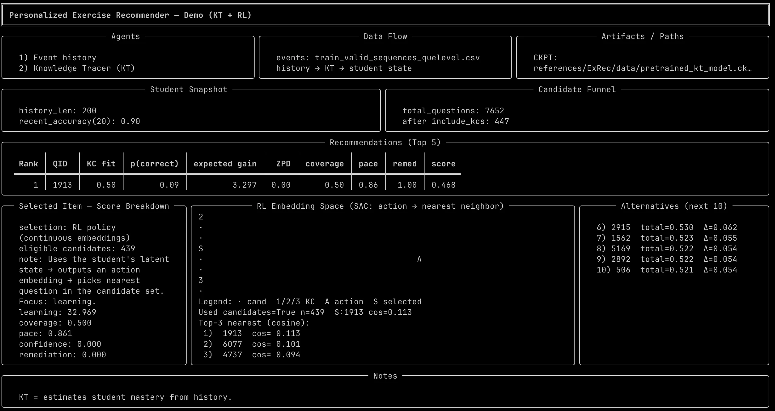
The demo shows:
- Student snapshot (mastery, weak KCs, recent accuracy)
- Candidate funnel (7,652 → filtered → scored)
- Top recommendations with score breakdowns
- RL embedding space visualization
What I Learned
1. Treat the KT model as an RL environment
This was the biggest conceptual shift. The knowledge tracing model isn't just a predictor—it's a simulator. You can ask it "what if the student answered this question correctly?" and get a new state back. That turns question selection into planning, and planning is what RL is good at.
2. Counterfactual simulation is surprisingly cheap
I expected simulating "correct" and "incorrect" outcomes for every candidate would be slow. It's not. The LSTM forward pass is fast, and you're not backpropagating. Scoring 200 candidates takes ~50ms on a laptop CPU.
3. Multi-objective scoring matters more than I thought
My first version just maximized expected learning gain. It kept recommending hard questions because those had the highest delta. Students got frustrated.
Adding coverage (don't repeat topics), speed (shorter questions when struggling), and confidence (stay in the ZPD) made the recommendations feel sensible. The weights are simple rules, not learned—but they work.
4. RL needs guardrails
The SAC policy sometimes outputs embeddings that map to weird questions—repeats, or items way outside the student's level. I added hard quality gates (no repeats, KC overlap, ZPD range) that run after RL selection. If the policy picks something bad, we either accept it anyway (and log it) or re-rank with stricter constraints.
This "RL proposes, rules dispose" pattern kept the system usable while the policy was still learning.
5. Cold-start is solved by embeddings
New students have no history, so the LSTM is at its default state. But you still have the question embeddings. You can recommend based on target KCs, difficulty proxies, or just sample randomly. The system degrades gracefully.
6. Latency budget drove architecture choices
Everything runs in a single forward pass per candidate. No database lookups in the hot path—embeddings are preloaded. The full pipeline (filter → score → select) runs under 100ms for 200 candidates. That's fast enough for interactive use.
7. The reward function is the hard part
KC-level mastery delta seemed like the obvious reward. But it's noisy—small state changes produce small rewards, and the policy has trouble learning. The exam-score reward (improvement on a sampled set of questions) was more stable, but required careful train/probe splits to avoid leaking evaluation into training.
8. Domain transfer is just data
The architecture doesn't care if questions are about math, medicine, or law. You need:
- Question embeddings (run BERT on your content)
- KC annotations (can be automated with LLMs)
- Interaction logs (student × question × correct/incorrect)
Swap those in, retrain the KT model, and the rest of the pipeline works.
What I'd do differently
- Start with heuristics: The greedy scorer (no RL) was good enough for 80% of cases. I should have validated it more before jumping to RL.
- Log everything: I added audit logging late. Should have done it from day one.
- Smaller action space: SAC in 768-dim embedding space works, but discrete actions (DQN over question indices) might converge faster for small question banks.
References
- Personalized Exercise Recommendation with Semantically-Grounded Knowledge Tracing (NeurIPS 2025)
- XES3G5M Dataset
- Tianshou RL Library
- pyKT Knowledge Tracing Toolkit
Built on math education data (XES3G5M), but the architecture works for any domain—medical, law, whatever. Just swap in your question bank and embeddings.